2 proofs in Information Theory: channel-convexity of mutual information¶

I've been studying Information Theory lately, through David MacKay's excellent book Information Theory, Inference, and Learning Algorithms. In it, there's an elementary Information Theory result left as an uncorrected exercise (Exercise 10.7), which could be phrased informally as: the Mutual Information is a convex function of the channel parameters.

In this article, I will give 2 proofs of this proposition:

The first proof uses typical calculus tools, proving convexity by computing the Hessian and showing that it's positive semi-definite.
The second proof only uses information-theoretical arguments.

The second proof is shorter, clearer, more insightful, and more self-contained. The first proof is the first one I delivered; it is longer and more technical.

So why write about the first proof at all? Because I see a few benefits to it:

It serves as a cautionary tale against always rushing to analytical methods, instead of searching for an insightful perspective on the problem.
From a pedagogical standpoint, it serves as an occasion to demonstrate how some classical tools from calculus and linear algebra can be used together.
If you're anything like me, you've always dreamt of knowing what the Hessian of Mutual Information looks like. (Come on, admit it.)

Problem statement¶

Background¶

Given two finite sets $X$ and $Y$, a discrete memoryless channel is a specification of probability distributions $P(y | x)$, for $x \in X$ and $y \in Y$.

Informally, this notion is motivated as follows: a sender chooses a message $x \in X$ to send, which after going through the communication channel will result in a receiver receiving some $y \in Y$. In an ideal world, we would be certain of what $y$ would be received after sending $x$ (in other words, y would be a function of $x$); but unfortunately, the channel adds random noise to the signal, such that after having chosen to send $x$, we only know the probability distribution $P(y | x)$ of what might be received.

Because the channel consists of $|X|$ probability distributions over a set of $Y$ elements, the channel can be represented by an $|Y| \times |X|$ transition matrix $Q$:

$$ Q_{yx} := P(y | x) $$

Therefore, each cell of $Q$ contains a values between 0 and 1, and the columns of Q sum to 1.

If we assume of probability distribution $P_X$ over $X$, a channel $Q$ gives us a probability distribution $P_Y$ of $Y$, by $P(y) = \sum_{x}{P(y | x)P(x)}$. Representing $P_X$ and $P_Y$ as vectors, this relation can be written as a matrix multiplication:

$$ P_Y = Q P_X $$

The mutual information $I[X;Y]$ between $X$ and $Y$ represents the average amount of information about $X$ that is gained by learning $Y$; phrased differently, it is the amount of uncertainty (entropy) about $X$ that goes away by learning $Y$. Formally:

$$ I[X;Y] = H[X] - H[X | Y] = H[Y] - H[Y | X] $$

In the above formula, $H[X]$ is the entropy of random variable $X$, and $H[X | Y]$ is the conditional entropy of $X$ given $Y$:

$$ H[Y] = \sum_{y}{P(y) \log(\frac{1}{P(y)})} $$$$ H[Y | X] = \sum_{x}{P(x) H[Y | X = x]} = \sum_{x}{P(x) \sum_{y}{P(y | x) \log(\frac{1}{P(y | x)})} } $$

What we want to prove¶

The result we want to prove is the following:

Given a probability distribution over $X$, the function $I: Q \mapsto I[X;Y]$ is convex.

In details, this means that given 2 channels $Q^{(0)}$ and $Q^{(1)}$, and a weight $\lambda \in [0,1]$, we can define a 'mixed' channel $Q^{(\lambda)} := \lambda Q^{(0)} + (1 - \lambda)Q^{(1)}$, with the property that $I(Q^{(\lambda)}) \leq \lambda I(Q^{(0)}) + (1 - \lambda)I(Q^{(1)})$

Intuitive interpretation¶

With regards to the capacity of conveying information, mixing 2 channels is always worse than using the most informative of the 2 channels we started with.

In particular, mixing 2 fully-deterministic channels (which are maximally informative) can result in a noisy channel!

Method 1: differentiation and Hessian¶

A common approach to proving that a function is convex is to differentiate it twice, yielding a Hessian matrix, and to prove that this Hessian is positive semidefinite. That's what we'll set out to do here.

Computing the Hessian¶

$I(Q)$ can be viewed as a function of $|X| \times |Y|$ variables, therefore our Hessian will be a square matrix containing $(|X||Y|)^2$ entries, of the form $\frac{\partial^2I}{\partial Q_{yx} \partial Q_{vu}}$.

To make calculations more lightweight, we'll use some shorthand notation:

$$ \pi_x := P(x) $$$$ \rho_y = \rho_y(Q) := P(y) $$

Recall that $\rho = Q \pi$, which can be reformulated to:

$$ \rho_y = \sum_{x}{Q_{yx} \pi_x} $$

As a result:

$$ \frac{\partial \rho_y}{\partial Q_{vu}} = \delta_{v = y} \pi_u $$

We now differentiate $H[Y]$ and $H[Y | X]$ with respect to $Q_{uv}$:

$$ \frac{\partial H[Y]}{\partial Q_{vu}} = \sum_{y}{\frac{\partial}{\partial Q_{vu}}\big\{\rho_y \log(\frac{1}{\rho_y})\big\}} = \sum_{y}{\frac{\partial \rho_y}{\partial Q_{vu}} \frac{\partial}{\partial \rho_y}\big\{- \rho_y \log(\rho_y)\big\}} $$$$ \frac{\partial H[Y]}{\partial Q_{vu}} = - \pi_u (1 + \log(\rho_y))$$$$ \frac{\partial H[Y | X]}{\partial Q_{vu}} = \sum_{x}{\pi_x \frac{\partial}{\partial Q_{vu}}H[Y | X = x]} = \pi_u \frac{\partial}{\partial Q_{vu}}H[Y | X = u] = \pi_u \frac{\partial}{\partial Q_{vu}}\big\{\sum_{y}{Q_{yu} \log(\frac{1}{Q_{yu}})}\big\}$$$$ \frac{\partial H[Y | X]}{\partial Q_{vu}} = - \pi_u (1 + \log(Q_{vu}))$$

Combining both results yields:

$$ \frac{\partial I(Q)}{\partial Q_{yx}} = \pi_x \log(\frac{Q_{yx}}{\rho_y})$$

Differentiating one more time, we obtain the entries of the Hessian:

$$ H_{(yx)(vu)} = \frac{\partial^2 I(Q)}{\partial Q_{yx} \partial Q_{vu}} = \delta_{x=u}\delta_{y=v} \frac{\pi_x}{Q_{yx}} - \delta_{y=v} \frac{\pi_x \pi_u}{\rho_y}$$

Proving the Hessian is positive semi-definite¶

Ordering the indices $yx$ in lexicographic order, thanks to the $\delta_{y=v}$ factor, we see that the Hessian matrix has a block-diagonal layout, with diagonal blocks $B^{(y)}$ of shape $|X| \times |X|$. It is therefore sufficient to prove that each diagonal block $B^{(y)}$ is positive semi-definite.

Denoting $\Delta := \text{diag}((\frac{\pi_x}{Q_{yx}})_{x \in X})$, we can write:

$$ B^{(y)} = \Delta - \frac{1}{\rho_y}\pi\pi^\top $$

We now prove that $B^{(y)}$ is positive semi-definite. Let $\epsilon$ a vector; we want to prove $\epsilon^\top B^{(y)} \epsilon \geq 0$.

$$ \epsilon^\top B^{(y)} \epsilon = \epsilon^\top \Delta \epsilon - \frac{1}{\rho_y} (\pi^\top \epsilon)^2$$

Therefore, our goal becomes to prove:

$$ \epsilon^\top \Delta \epsilon \geq \frac{1}{\rho_y} (\pi^\top \epsilon)^2 $$$$ \Uparrow $$$$ (\pi^\top \epsilon)^2 \leq \rho_y (\epsilon^\top \Delta \epsilon)$$$$ \Uparrow $$$$ \big(\sum_{x}{\pi_x \epsilon_x}\big)^2 \leq \big(\sum_{x}{Q_{yx} \pi_x}\big) \big(\sum_{x}{\frac{\pi_x}{Q_{yx}} \epsilon_x^2}\big) $$

So we want to compare a squared sum of products to a product of two sums... this looks like a job for the good old Cauchy-Schwartz inequality! And indeed, observing that $\pi_x \epsilon_x = (\sqrt{Q_{yx} \pi_x})\big(\sqrt{\frac{\pi_x}{Q_{yx}}} \epsilon_x \big)$, it is easily verified that the Cauchy-Schwartz inequality yields the desired result.

Some justifications regarding domains of validity¶

Looking at the above derivation, you may want to object as to the validity of certain derivations. I'll try to make the required justifications here:

You treated $I(Q)$ as a function of $|X||Y|$ unconstrained variables, whereas it's really defined on an $|X|(|Y| - 1)$-dimensional polytope, because of the constraints on the columns sums.

True, but it doesn't hurt to extend the domain of definition of $I(Q)$ - if the extended function is convex, so is its restriction to values of $Q$ that are truly channels.

To differentiate, you have assumed that $Q_{yx}$ is non-zero.

Indeed; we prove the convexity of $I$ to the (dense, open and convex) subset of $Q$s where that's true, and can then conclude $I$ is convex on its entire domain using a continuity argument.

To differentiate, you have assumed that $\rho_y$ is non-zero.

True; however, observe that this assumption is valid provided that all $Q_{yx}$ are non-zero.

Method 2: an elegant, idiomatic proof¶

We now revisit the notion of "mixing two channels", by interpreting the mixing coefficients themselves as probabilities.

We denote $Q^{(\lambda)} := \lambda Q^{(1)} + (1 - \lambda) Q^{(0)}$.

Consider the following protocol of communication. When we send message $x$, a random $z \in \{0, 1\}$ is independently generated, with $P(z=1) = \lambda$: if $z = 0$, $x$ is sent through channel $Q^{(0)}$, otherwise through channel $Q^{(1)}$.

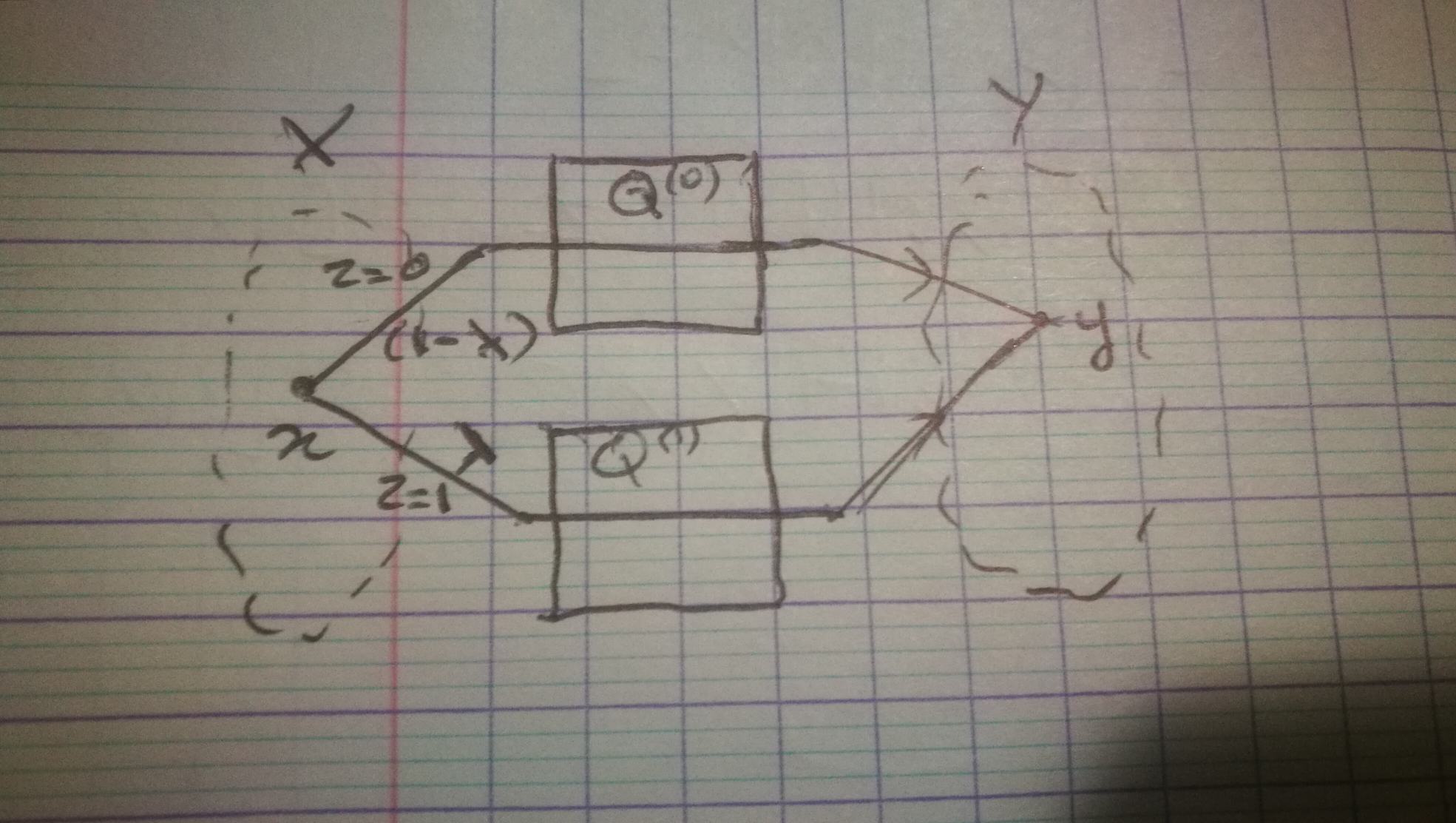
We can verify that this 'composite' communication channel is exactly equivalent to $Q^{(\lambda)}$:

$$ P(y | x) = P(y, z=0 | x) + P(y, z=0 | x) = P(z=0)P(y|x, z=0) + P(z=1)P(y|x, z=1) $$$$ P(y | x) = (1 - \lambda)Q^{(0)}_{yx} + \lambda Q^{(1)}_{yx} = Q^{(\lambda)}_{yx}$$

We can now derive the proof by starting with an incredibly intuitive argument: knowing both $y$ and $z$ gives us more information on $x$ than knowing $y$ alone. Formally:

$$ H[X | Y, Z] \leq H[X | Y] $$$$ \Downarrow $$$$ P(z = 0)H[X | Y, z = 0] + P(z = 1)H[X | Y, z = 1] \leq H[X | Y] $$$$ \Downarrow $$$$ (1 - \lambda)H[X | Y](Q^{(0)}) + \lambda H[X | Y](Q^{(1)}) \leq H[X | Y](Q^{(\lambda)}) $$$$ \Downarrow $$$$ (1 - \lambda)(H[X] - H[X | Y](Q^{(0)})) + \lambda (H[X] - H[X | Y](Q^{(1)})) \geq (H[X] - H[X | Y](Q^{(\lambda)})) $$$$ \Downarrow $$$$ (1 - \lambda)I[X ; Y](Q^{(0)}) + \lambda I[X ; Y](Q^{(1)}) \geq I[X ; Y](Q^{(\lambda)}) $$

The last line expresses the convexity of $I(Q)$. QED.